Bendix tutorial
Contents:
Overview of the Bendix graphical user interface and its settings
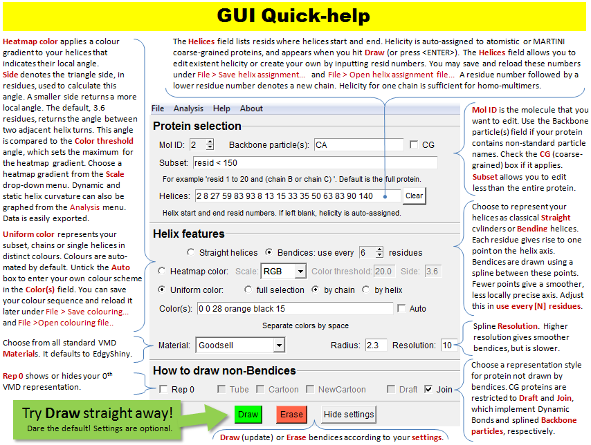
This image is also available under Bendix'
Help > Quick Help.
Bendix at a glance
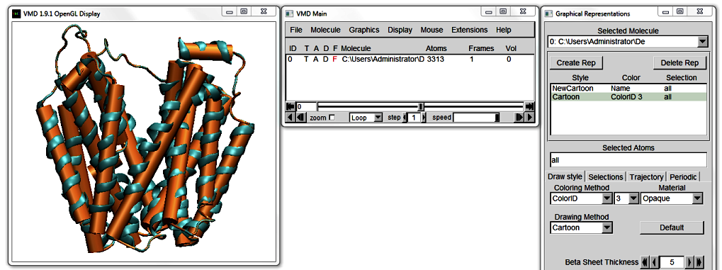
1. Existent helix representations.
Start VMD and load 1PV7_LacY.pdb. In VMD's Main window, go to
Graphics > Representations... to open the Graphical Representations window. In the Drawing Method pull down menu, select NewCartoon. The Display updates to show this representation.
At the top of the Graphical Representations window, click Create Rep. Change the Drawing Method of your new Representation to Cartoon, and the Coloring Method to ColorID to distinguish between the two representations. Pick a colour of your choice from the drop-down menu. Notice how each colour is numbered.
Move the protein around. The straight Cartoon cylinders work well as a high-level abstraction of the protein, but they do not do justice to curving helices. The NewCartoon ribbons, on the other hand,
show the backbone projection, which gives a very detailed view of a helix in any conformation.
Bendix is a middleground between these two Drawing Methods; it combines the level of abstraction of Cartoons with the conformational detail of NewCartoon.
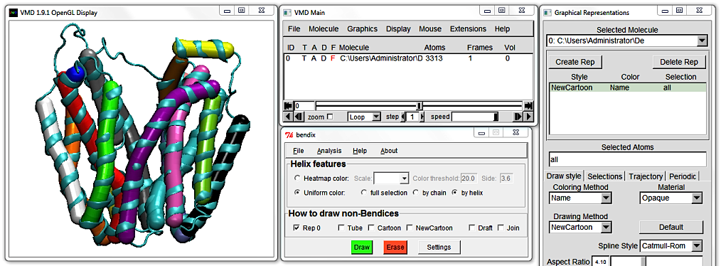
2. Easy and functional helix abstraction in Bendix.
Delete the Cartoon Representation and open Bendix from
VMD Main > Extensions > Analysis > Bendix.
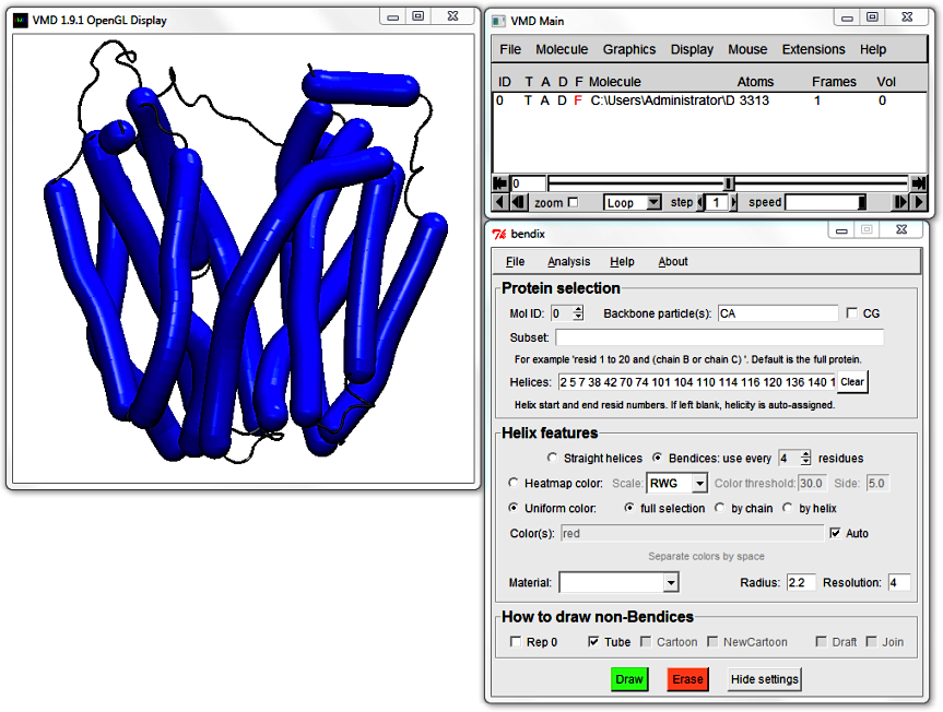
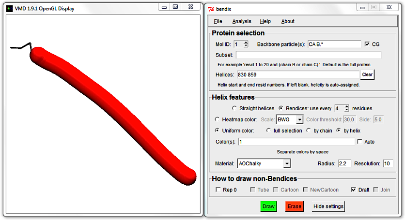
Keep the default settings and click the bottom green
Draw button, alternatively press
Enter on your keyboard. Either of these actions updates the screen but we will use
Enter in the remainder of this tutorial.
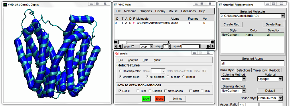
This is the Uniform colour scheme. Notice how the Bendix helix abstractions - we'll call them "bendices" from now on, to distinguish between representations - approximate the helices' conformation.
The bendix algorithm works by calculating and graphing the axis that goes through the spiralling helix backbone. To fit the bendices even closer to the helix axis, or alternatively, to achieve smoother axes, read on or jump straight
to The tutorial section on spline settings.
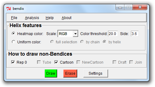
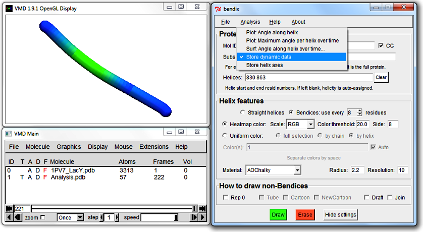
3. A closer look at the Bendix window
At the top of the window is a menu bar, wherefrom you can load and save settings, analyse your protein and get help with Bendix.
Below is a section called Helix features, where you can switch between uniform colouring (which you are currently viewing) and analytical, angle-indicative colouring of bendices.
Their settings are shown on their right hand side.
Next follows the How to draw non-Bendices field, which is responsible for updating the parts of your protein that you do not choose to portray as bendices, such as beta sheets and coil secondary structure,
or what is left of your protein when you choose to only Bendix-display a subset of it (more on this later).
At the bottom of the window are the three buttons Draw, Erase and Settings. You have used Draw already (or its keyboard counterpart, Enter) to execute Bendix settings.
Erase erases all things drawn using Bendix and Settings displays advanced Bendix settings.
You are currently viewing LacY using uniform, individual helix colouring. To colour in the full protein uniformly, tick
full selection and press
Enter (or click the green
Draw button)
to execute the settings. All bendices turn blue. The
by chain option is applicable to multimeric proteins.
5. Helix features: Heatmap color
Now change to angle-indicative graphics by ticking Heatmap color and pressing Enter. Your protein appearance changes to indicate helix geometry using a heatmap colour scheme.
The default colour scheme, which you are viewing, is RGB or Red-Green-Blue. Red indicates the areas of highest helix axis angle, followed by green for intermediate angle magnitudes and blue for angles close to,
or at 0 degrees. Bendices' ends are at angle 0 per definition, since they are not resolved by the axis-generating algorithm. For more information about the precision of the Bendix' algorithm, please see Technical detail under the faq section.
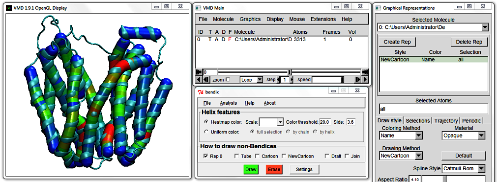
You can change the threshold at which an angle is displayed as a maximum angle colour by editing the Colour threshold value. It is set at 20 degrees by default, which means that any helix angle at or above 20 degrees is graphed in red.
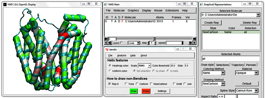
Increase this to 30 and hit Enter. By increasing the threshold, less helices make the cut, and only highly curved helix-areas remain red. By tuning this threshold until no or little red remains, you can get a good first idea of how curved your helices are.
Change the Colour threshold to 10, and note how less curved helices now display red areas, as only a 10 degree angle is necessary to qualify. If your helices are not particularly curved,
you can thus still tune the Colour Threshold to emphasize existent curvature.
The Scale drop down menu lets you choose between different VMD colour gradients for your helix angle display. Click it to display available gradients, and pick a gradient of your choice.
The bottom choices, BlkW and WBlk are black and white gradients that are good for black and white publishing.
Rightmost is the Side setting. This is the side length, in residues, of the angle used to measure helix curvature.
Since the angle is measured between two sides, your helix of interest needs to be at least twice the chosen angle side length to allow analysis.
The default value, 3.6, denotes the angle between two adjacent alpha helical turns, so requires a helix to be approximately 8 residues long to compute.
Smaller helices are 0-angle coloured and do not feature in analysis graphs (more on this in the Analysis section).
Vary Side to see its effect on LacY. Note that a small angle side measures local helix angles, whereas a large angle side measures global helix curvature.
For the purpose of this tutorial, choose Uniform color, full selection and hit Enter.
6. How to draw non-Bendices
Rep 0 displays (ticked) or hides (untick) the zeroth Graphical representation of your protein,
if you have one. In our case, the zeroth representation is the NewCartoon Representation. Untick this box to hide this representation.
Now only bendices are displayed. Use the adjacent three tick-boxes to link them up. Untick your former representation choice to make a new choice.
You will notice that a new row appears in the Graphical Representations window as you move between the renditions of LacY's coiled coil regions. This allows you to change e.g. the representation's colour and resolution.

Customization
1. Advanced settings
Click the
Settings button on the bottom left of the Bendix window. The Bendix window expands, revealing more settings.
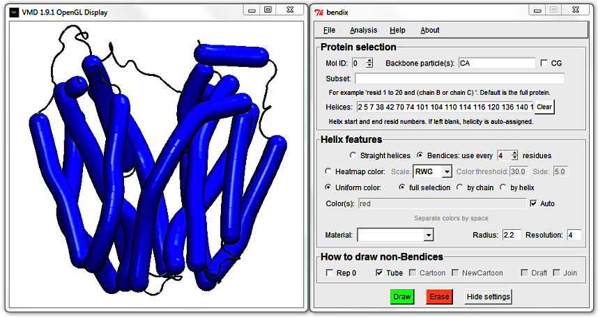
2. Protein selection
The new top field allows you to control which helices are displayed as bendices. Use Mol ID to choose between available, loaded molecules.
At the moment the only loaded molecule is LacY, and it's ID is 0.
To the right is the Backbone particle(s) field that allows you to specify the particle names that Bendix will search for when rendering non-bendices. This is useful if your molecule consists of non-standard particles. Rightmost is the CG tickbox that allows you to specify whether your protein is coarse-grained, which enables coarse-grained settings, including alternative backbone particle names. We will return to these settings later.
The Subset field allows you to choose to render only part of your molecule using Bendix. If you leave it blank, it renders all. The Subset field works in conjunction with the Helices field, underneath.
The Helices: field writes out the Subset's helicity so that you can edit it. At the moment it displays helicity for all of LacY.
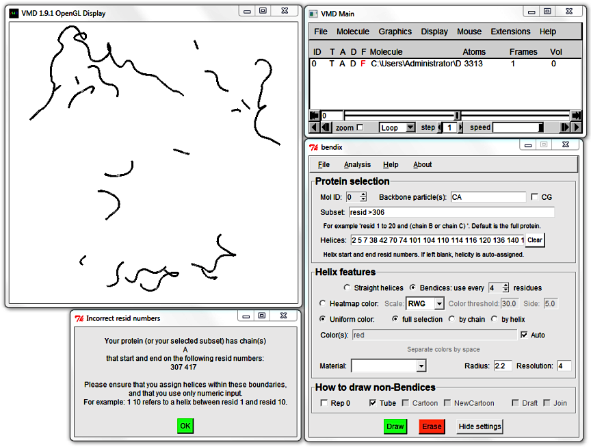
Try the Subset field using standard VMD syntax. Choose to only Bendify residue numbers above 305 by writing
resid >305
and hitting Enter.
An error message appears. Bendix detected that your chosen helicity (in the Helices field) does not match your Subset. The two fields need to match for Bendix to work.
Click OK in this message and the subsequent one. Leave your Subset field intact (it should still read resid >305),
hit the Clear button next to the Helices field and execute your settings using Enter.
This allows Bendix to query STRIDE for your Subset's helicity and update your screen.
3. Edit helicity
As just mentioned, the helicity written out in the
Helices field is calculated by the program STRIDE (Frishman D & Argos P (1995) Proteins 23:566).
Delete the first helix by editing out its start and stop residue numbers. Afterwards, the
Helices field should look like this:
343 355 357 375 378 398 408 416
Hit Enter and explore the available respresentations under How to draw non-Bendices. Tube, Cartoon, NewCartoon and Draft are ported straight from VMD's standard arsenal of representations. Draft is a DynamicBonds treatment of Backbone particle(s). Join is representation that also work on supplied Backbone particle(s), but which has an in-built, smoothing Hermite spline and joins up bendices to their backbone (standard VMD representations may leave small gaps). It also incorporates NewCartoon's beta sheets for atomistic proteins and draws arrows for CG Martini proteins as they are not supported by NewCartoon.
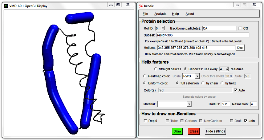
The large helix is broken in two. You can mend it by editing the numbers in the Helices field,
deleting the end residue number of the first helix and the start residue number of the second helix that you wish to fuse.
But how do you know which numbers to delete? Bendix features a straight-forward way to identify what start and stop resids belong to which helix.
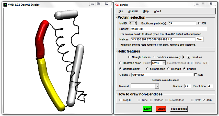
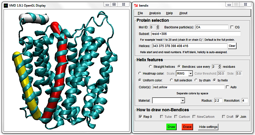
In the Helix features section of the extended Bendix window, choose Uniform color: by helix. Immediately underneath is the Color(s) field.
It is currently disabled as colours are automatically generated. Activate the field by unticking the Auto box to the right. Note that red is listed by default; keep this default and hit Enter.
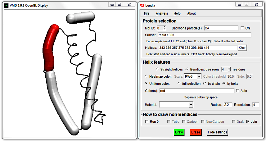
The Display updates to show the first bendix in red. Since the first helix listed in the Helices: field has start residue number 343 and ends at residue number 355, we now know that those belong to the red helix.
The next helix starts already at residue 357, so this is probably the junction that we want to mend. To convince yourself, edit the Color(s) field by adding a second colour of your choice
(beware, colours are spelled in American English). As noted previously, VMD colours are listed alongside numbers in Graphical Representations' drop-down list of ColorIDs.
You can use these numerical colour IDs in the place of colour words. As always, hit Enter to execute.
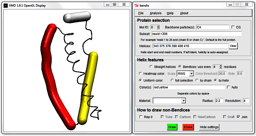
To do the helix fusion, locate the end of the first helix (355) and the start of the adjacent helix (357) and delete them. Hit Enter to update the display and note how the two close, adjacent helices are now merged.
Also, the Color(s) that you chose have been redistributed to their new corresponding helices.
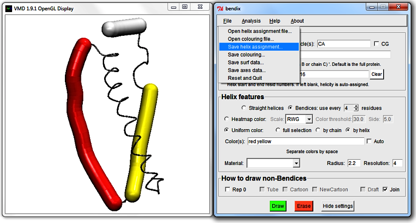
4. Save edited helicity
If you grow fond of your own custom sequence of
Helices or
Color(s), both can be saved and reloaded under
File in the Bendix menu.
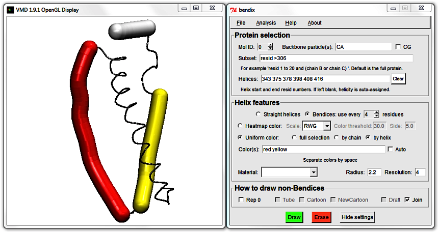
5. Helix features: Straight helices and spline settings
In the Helix features section, you can choose to graph your helices as straight cylinders.
This is already implemented in VMD for atomistic proteins, but is valuable to have for coarse-grained proteins, not least because they are computationally cheap to draw
(N.B. that everything demonstrated in this tutorial is also available for coarse-grained proteins).
Next to the Straight helices option is Bendices, the default rendering mode. It comes with the setting use every [N] residues, where [N] refers to the set value.
This setting controls the spline used to generate bendices. The algorithm that computes the helix axis generates one point per residue; use every [N] residues controls how many of these points are used.
The more residues' axis points that you use (a low N value), the closer the fit to the helix axis. Alternatively, for a smoother helix, use fewer points (a higher N value).
The default setting, 4, saves approximately one point per helix turn.
For more info on the Bendix spline algorithm, see Technical detail under the faq section.
Try changing the use every [N] residues setting to see what it does to the bendices' projections.
Compare this to the NewCartoon representation by ticking the Rep 0 tickbox in the bottom left corner of the Bendix window.
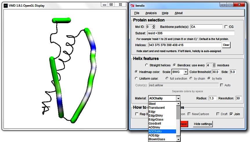
6. Helix features' final touches: Material, resolution and radius
Return use every [N] residues to 4 and choose to Heatmap color using your favourite heatmap gradient. At the bottom of the Helix features field,
you can explore what VMD Material to use. The adjacent Radius setting sets the radius of bendices (in Angstrom).
Resolution sets how many spline points to use per point saved by use every [N] residues. Higher Resolution gives smoother bendices, but takes more time to draw.
Remember that you always can look at the Quick Help image, which explains all Bendix fields, and is available in Bendix under Help > Quick Help.
Analysis
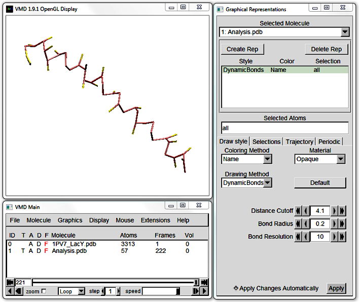
1. VMD visualization of coarse-grained particles
Reduce LacY's Resolution to 10 and open Analysis.pdb and Analysis.dcd in VMD. This is a helical, coarse-grained (CG) peptide (using the MARTINI force field) and its trajectory.
The default VMD visualisation of CG proteins is difficult to make out,
but you can approximate the protein backbone by using DynamicBonds as Drawing Method under Graphics > Representations.
Increase the Distance Cutoff until the peptide appears (circa 4). However, beware that this algorithm draws bonds between all points within the Cutoff, whether or not they are bonded.
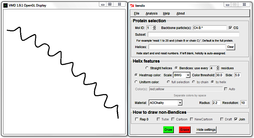
2. Prepare Bendix for a new molecule
If you did not delete LacY prior to loading Analysis.pdb, increase the Mol ID to 1 to reflect Analysis.pdb's ID, and clear Subset and Helices fields.
3. Bendix visualization of coarse-grained particles
Hit Enter. If Stride-related Error messages appear in the Terminal, do not fret - Stride is automatically called to calculate the secondary structure of loaded proteins,
but fail to do so for coarse-grained proteins as STRIDE wasn't developed for these particle types.
Tinker with Bendix settings such as Material, Resolution and colouring to convince yourself that all previously mentioned settings work equally well for CG proteins.
The only novelty in the Bendix window is found in the How to draw non-Bendices section, where representations for atomistic representations are grayed out.
As this peptide is all-helical, the remaining representations will not render anything. To see their effect, Clear the Helices field and try out Draft and Join.
Join draws a spline and joins backbone and bendices whereas Draft bonds anything within a cutoff with straight lines. When you graph larger molecules than this peptide, you will notice that Join renders slower than Draft, since you pay in CPU time for the extra computed detail.
Untick Join and Draft and hit Enter to generate a bendix again. Reduce its length by editing the Helices field, hit Enter and then tick the Draft tickbox.
4. Analyse a static peptide's local angles along the length of the helix.
Change the
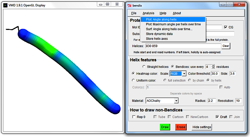
Resolution to 10 and choose to
Heatmap color,
use every 4 residues and using
angle
Side: 3.6.
It is necessary to graph your protein using the angle colour scheme prior to analysing it. Besides, options under the
Analysis menu will remain inactive until you do so. Hit
Enter.
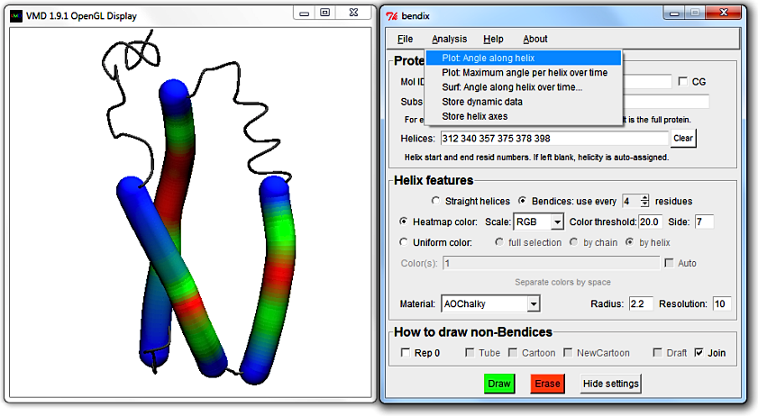
In the Bendix menu, go to Analysis > Plot: Angle along helix.
Bendix uses Multiplot (by Jan Saam, with contributions from Kohlmeyer, Lederer and Gumbart) for its scatter plots.
Along the x-axis is the length of the helix and the y-axis shows the helix axis' curvature in degrees.
Note that the peripheral first and last circa four residues show perfectly linearly increasing and decreasing, respectively, local angles.
This is artificial; the local angle at first and last circa four residues can not possiby be calculated as the angle Side is 3.6 residue lengths long.
Instead helix start residues 1 to 4.6 are given values from 0 degrees to the first measured angle at circa
residue 4.6.
The linear angle values do not hit residue 4.6 precisely at this Resolution;
you will find that as you increase Resolution,
the helix axis becomes more densely populated with spline points
so that the line end will approximate residue 4.6 better.
The helix end is treated the same way, but with a decreasing angle gradient.
N.B. you can hover over a Multiplot datapoint to display its value in the Terminal.
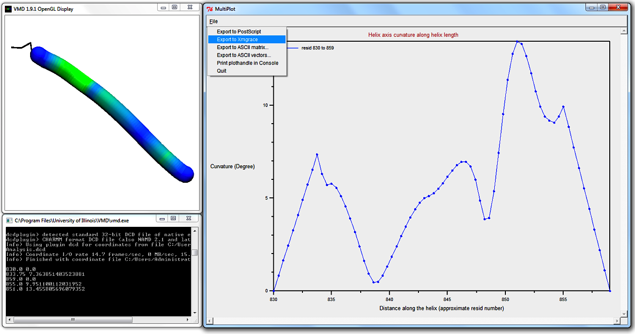
The graph shows several low-curvature peaks, whereof the highest curvature is found approximately three quarters of the way to the C-terminus.
Compare this plot to the heatmap-coloured bendix in the VMD Display, assuring yourself that its heatmap is correct.
To distinguish better between heatmap maxima and minima, you can alter the Colour threshold.
Hovering over the maximum angle data point in the Multiplot, we deduce that the highest curvature is ~13.5 degrees, so it is advisable to adjust the Colour threshold to approximate this value.
Color threshold only changes the helix heatmap display; it does not change the Multiplot graph.
Note that you have the option to export your data in the top left-hand corner in MultiPlot's File-menu.
5. Analyse a static protein's local angles along the length of several helices.
Several static helices' curvatures can be plotted simultaneously for easy comparison. Return to LacY by making it the Top molecule and pressing
= in the Display window to update the view (after making the helix top, you can also reset the view from
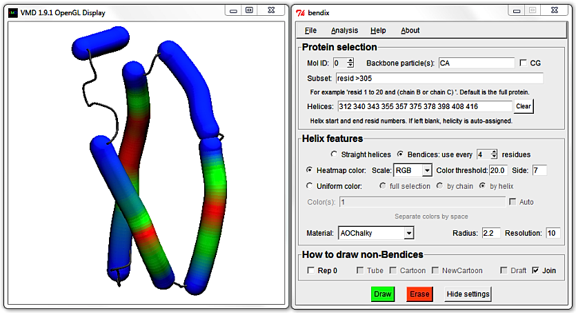
VMD Main > Display > Reset View). Use the previous
Subset,
resid >305
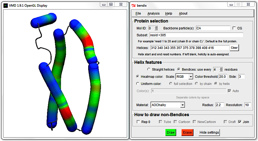
Select Heatmap color, use every 4 residues, Side 7, the default Color threshold 20 and Scale RGB, and then hit Enter.
As before, this subset should generate these Helices:
312 340 343 355 357 375 378 398 408 416
Three helices are drawn using angle-indicative heatmap graphics and two smaller helices are drawn using uniform zero angle colour (in RGB's case, the zero-angle colour is blue).
The latter indicates that the helix contains too few residues to measure its angles using Side 7 residue lengths, which demands a minimum of 15 residues to compute.
This has implications for MultiPlot, where only qualifying helices are graphed.
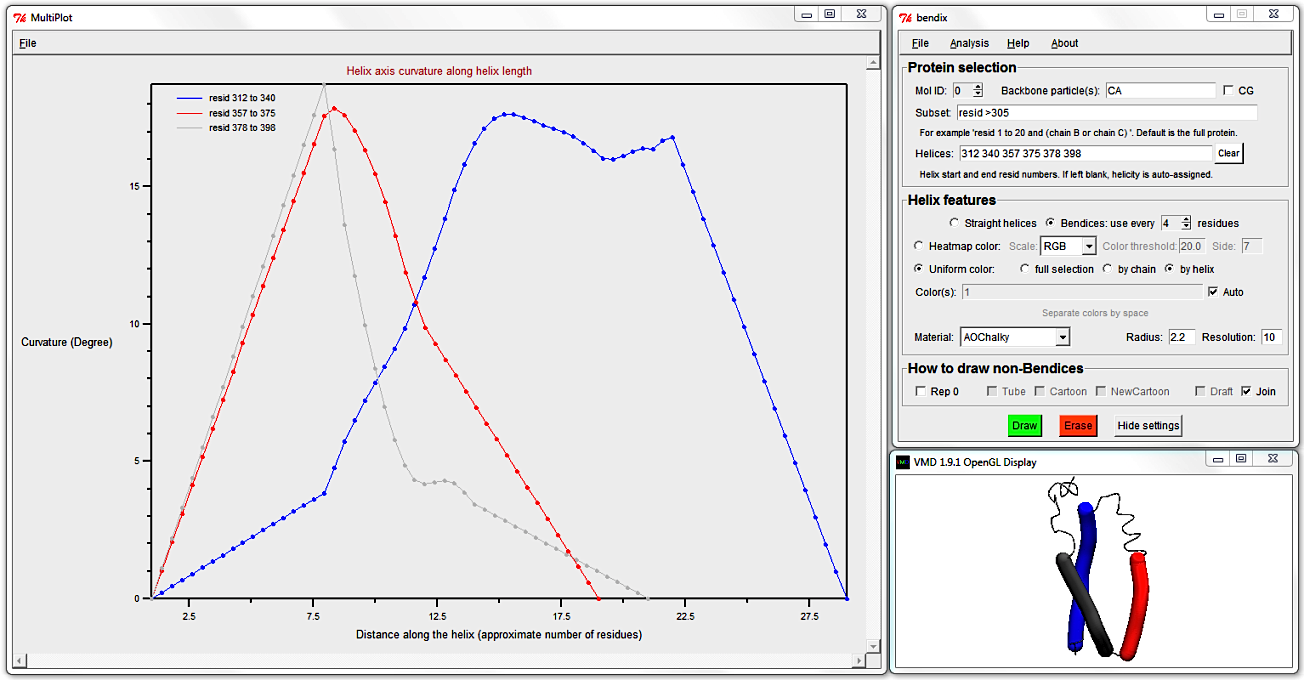
Identify the helices that are shorter than 15 residues in the Helices field and remove them. The result should read:
312 340 357 375 378 398
Go to Analysis > Plot: Angle along helix again. The top left legend shows which trace corresponds to which helix residues.
Another way to reveal the trace-helix correlation is to exploit that Multiplot trace colours were set up to correspond to the automatic uniform colour sequence.
That way you can intuitively see which trace belongs to which helix. To use this, keep the Multiplot graph open while selecting Uniform color, by helix option back in the Bendix window.
Tick the Auto box next to the Color(s) field and hit Enter.
Now each helix colour corresponds to its respective trace colour in MultiPlot.
Note that in order to obtain this colour correspondence, helices that are so short that their angles can't be evaluated have to be removed, or they will scramble the colour sequence.
A word of warning: only the first six automatic colours correspond to Multiplot trace colours. Secondly, Multiplot trace colours repeat after 26 helices are graphed. Graph fewer helices to overcome these problems.
To target shorter helices, evaluate more local angles by using a smaller angle Side.
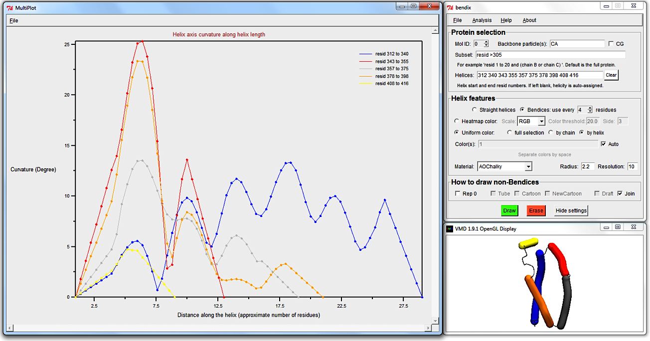
Clear the Helices: field (else your own helicity will override STRIDE's assignment) and select Heatmap color, Side 3 and hit Enter.
This small angle Side evaluates the angle within a single alpha helical turn,
so allows analysis of even the smallest helix in our Subset.
For more info on the angle algorithm, see the Technical detail under the faq section.
Use MultiPlot to graph the local angles along each helix and, seeing as we're dealing with six or fewer helices, you can derive which helix corresponds to which trace using the automatic uniform colouring, as demonstrated previously.
To move the Multiplot legend out of the way of traces, just click and drag it to a new position.
Smoother Multiplot traces can be obtained by increasing the spline point density by increasing Resolution.
6. Analyse how local helix distortion along the length of the helix evolves over time: general advice
Return to the single CG peptide. Deleting LacY will take you back to the CG helix view immediately,
but if you wish to hold on to LacY, you can return to the CG helix by making it the Top molecule and pressing
= in the Display window to update the view (after making the helix top, you can also reset the view from
VMD Main > Display > Reset View).
Pressing
= at any point when you view your surf graph (see
below) will also reset
the viewpoint to the original perspective.
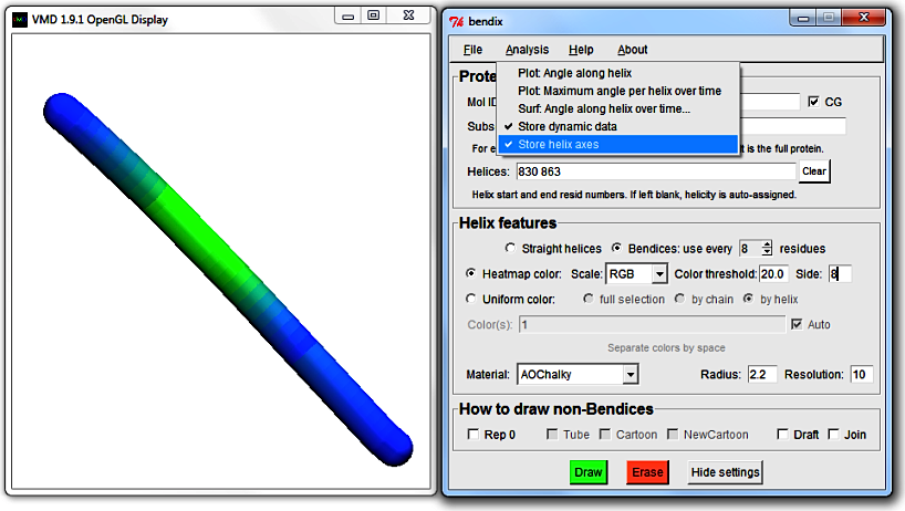
Select Heatmap color, use every 8 residues, Side 8, Resolution 10, and hit Enter.
By default, to speed up Bendix helix display, local angles along the length of the helix are only stored for the current frame (and only if rendered using Heatmap color).
To graph dynamic data, tick Store dynamic data which is found under Bendix' Analysis menu. Now each frame's helix curvature gets stored as you play your trajectory.
This requires memory and will eventually slow your frame rate.
Frame rate depends on the number of datapoints stored, which is correlated with Resolution, number of frames, helix length and number of helices, and inversely correlated with use every [N] residues and Side.
Reduced frame rate is necessary if you wish to graph helix geometry over time.
Angles corresponding to a specific frame are not evaluated until that frame is displayed using Bendix' angle-indicative rendering. Therefore you need to play your trajectory before analysis of dynamics becomes available.
Correspondingly, dragging the VMD frame-indicator rapidly through the trajectory will result in datapoints only for those fragmentary frames that are drawn to screen.
The Play button, using step 1, ensures that data for each frame is stored. Stored angle data is deleted when you hit Erase, or upon return to Frame 0, so if you intend to graph your data,
be sure to prevent your trajectory from returning to Frame 0. You can do this by changing the default 'Loop' play mode to 'Once' at the bottom of the VMD Main window.
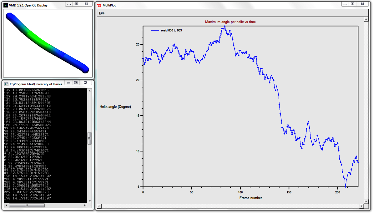
7. Analyse how the local helix distortion along the length of the helix evolves over time: Maximum angle
Press Play to see the evolution of the CG helix conformation over time.
At the end of the trajectory, go to the Bendix'
Analysis > Plot: Maximum angle per helix
over time. The result MultiPlot graph shows how the helix' maximum curvature curvature, per frame,
changes over time. This graph shows that the helix undergoes sigificant straightening,
as the maximum angle per frame is reduced from a maximum of 27.575 degrees to minimum 4.987 degrees (recall that hovering over a
datapoint displays its value in the Terminal).
As mentioned previously, MultiPlot allows data export.
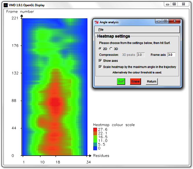
8. Analyse how the local helix distortion along the length of the helix evolves over time: Surf
Bendix has a built-in module that graphs saved dynamic helix distortion in the
VMD Display window.
Go to Bendix'
Analysis > Surf: Angle along helix over time...
The
Angle analysis window appears, and the VMD Display is cleared
(upon window closing, all other loaded molecules will reappear).
The Angle analysis window has a menu wherefrom you may save datapoints
or quit.
 The Angle analysis window features settings to control graph display:
In 2D heatmaps, angle magnitude is presented using your chosen colour scale gradient.
Angle data can also be viewed using a 3D landscape. Compression allows more compact data display of data.
This is beneficial if you wish to condense a long trajectory into a lucid graph that fits the page,
or scale 3D peaks up or down. Show axes does what it says on the tin, and also generates a colour scale bar for the 2D
heatmap to aid visual angle quantification. Scale heatmap by the maximum angle in the trajectory
is ticked by default. It takes into account the maximum angle computed during the trajectory (in this case ~27.5 degrees)
and uses this as the Colour threshold to scale the heatmap accordingly.
Untick this box to graph using the Colour threshold specified in the Bendix main window.
The green Surf button executes your settings (like Draw does in the main window),
Erase and Return both erase angle analysis graphics,
but Return also closes the Angle analysis window and returns you
to the former protein viewpoint.
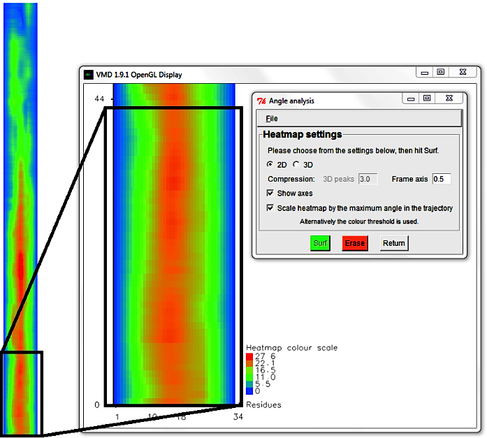
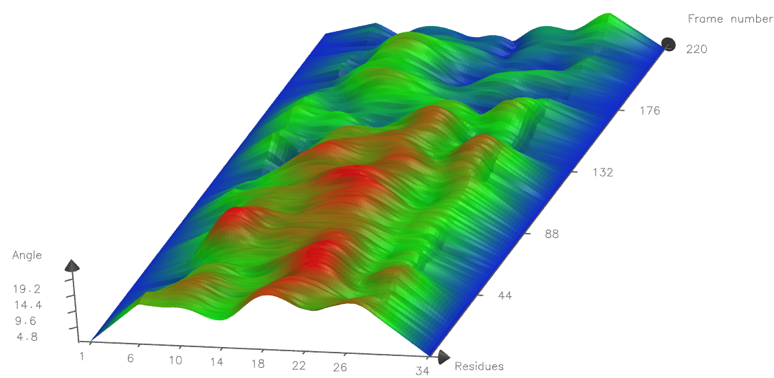
Leave the default 2D setting and hit Surf. A 2D heatmap appears.
You may wish to angle the graph slightly to get better colour contrast
(click R in the Display window to rotate the graph).
Click Show axes to display axes.
The horizontal axis displays the length of the helix, in residues, and the vertical axis shows trajectory time.
Residue number spacing is uneven as only residues that are mapped to a certain point
along the axis are plotted. You may choose what residues to map in the Bendix main window's setting
use every [N] residues. Helix start and end residues are mapped by default.
To read more about Bendix' precision, see Technical detail under the faq section.
On the vertical 'time' axis, each horizonal row represents the curvature along the helix,
per trajectory frame. Higher up rows display helix distortion further along in time.
Helix curvature magnitude is expressed by heatmap that is quantified in the Heatmap colour scale bar
on the right.
The Angle analysis window features settings to control graph display:
In 2D heatmaps, angle magnitude is presented using your chosen colour scale gradient.
Angle data can also be viewed using a 3D landscape. Compression allows more compact data display of data.
This is beneficial if you wish to condense a long trajectory into a lucid graph that fits the page,
or scale 3D peaks up or down. Show axes does what it says on the tin, and also generates a colour scale bar for the 2D
heatmap to aid visual angle quantification. Scale heatmap by the maximum angle in the trajectory
is ticked by default. It takes into account the maximum angle computed during the trajectory (in this case ~27.5 degrees)
and uses this as the Colour threshold to scale the heatmap accordingly.
Untick this box to graph using the Colour threshold specified in the Bendix main window.
The green Surf button executes your settings (like Draw does in the main window),
Erase and Return both erase angle analysis graphics,
but Return also closes the Angle analysis window and returns you
to the former protein viewpoint.
Leave the default 2D setting and hit Surf. A 2D heatmap appears.
You may wish to angle the graph slightly to get better colour contrast
(click R in the Display window to rotate the graph).
Click Show axes to display axes.
The horizontal axis displays the length of the helix, in residues, and the vertical axis shows trajectory time.
Residue number spacing is uneven as only residues that are mapped to a certain point
along the axis are plotted. You may choose what residues to map in the Bendix main window's setting
use every [N] residues. Helix start and end residues are mapped by default.
To read more about Bendix' precision, see Technical detail under the faq section.
On the vertical 'time' axis, each horizonal row represents the curvature along the helix,
per trajectory frame. Higher up rows display helix distortion further along in time.
Helix curvature magnitude is expressed by heatmap that is quantified in the Heatmap colour scale bar
on the right.
Hit Erase and edit the Frame axis compression to 6.0.
Select Draw and Show axes to display a more concise graph.
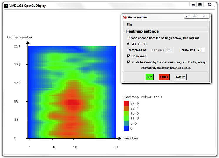
Alternatively hit Erase and change the Frame axis compression to 0.5 to
zoom in and resolve individual trajectory frames.
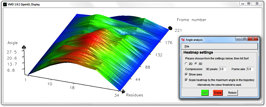
Hit Erase and swap to the 3D surf option, using a Frame axis compression of 5.0.
When the display updates, rotate the graph (by typing 'r' in the Display and using the mouse)
until the surface displays well.
If the graph is 'cut' as you approach it, it's because of your clipping plane settings.
To modify the clipping plane, ensure that the Display window is active,
type T to get to Translate Mode and, holding down your right mouse button,
drag the cursor left or right (you can also reach these mouse function settings from the
VMD Main window under the Mouse menu).
The clipping plane can also be edited from VMD Main > Display > Display Settings...
by changing Near Clip and Far Clip.
Reducing the Near Clip to 0.00 will display more of your near field of view.
The 3D graph benefits from the extra dimension to display angle distortion magnitude.
The angles along the helix length of the very first frame is shown clearly as the graph contour
along the Residues axis.
The same graph is obtained by using Analysis > Plot: Angle along helix on the first
static frame.
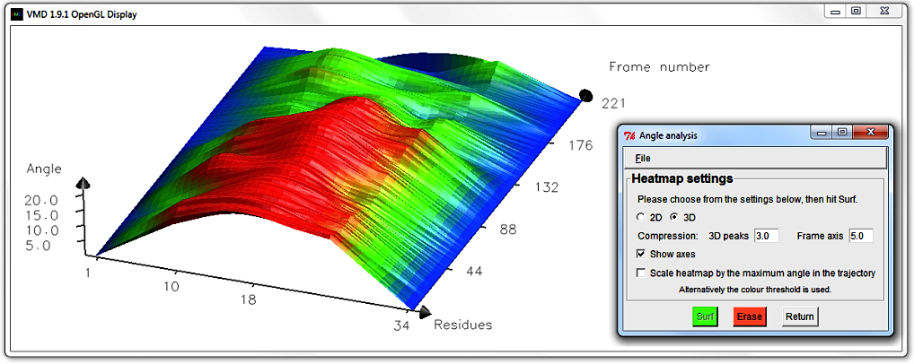
Untick the Scale heatmap by the maximum angle in the trajectory box.
The Display updates automatically to show the same surface shape,
but where the angle-indicative colour scheme has been scaled to the value in the Bendix window's
Colour threshold; in our case 20.0 degrees.
The Angle axis is altered to reflect this new maximum; in our case it has contracted.
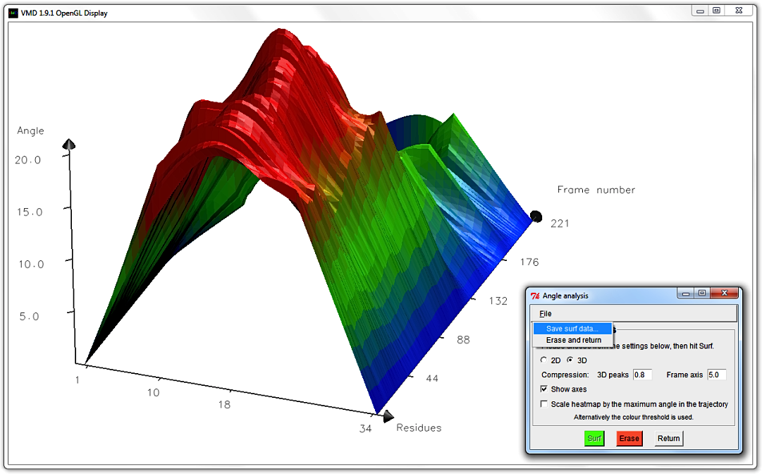
To get more surface altitude contrast, hit Erase and edit the 3D peak compression to 0.8.
Hit Surf. An amplified graph appears with scaled up, emphasized peaks.
N.B. Angle analysis settings only alter how the surface is rendered in the VMD Display.
It doesn't alter the data.
Lastly, you can alter what Material your graph is drawn with in the main Bendix window,
and if you wish to capture your graph, standard VMD molecule rendering applies
(it can be found under VMD Main > File > Render...).
Below is an example of a Tachyon rendered graph of the same peptide, using Resolution 15, use every 4 residues, Side 5 and Material AOChalky. Note the more closely spaced residue numbers on the X-axis, reflecting use every 4 residues compared to use every 8 residues used in the example above. The curvature profile is also different since a more local angle is measured (the angle Side is 5, compared to 8 as above).
Go to File in the menu and select Save surf data....
A window pops up that asks you to provide a File name and folder destination for your 3D data.
Save the data using an extension that allows you to open it in a text editor, e.g. .txt.
Open the file. The header explains how the file layout.
This tabbed data can be copied straight into alternative graphing softwares, such as MatLab.
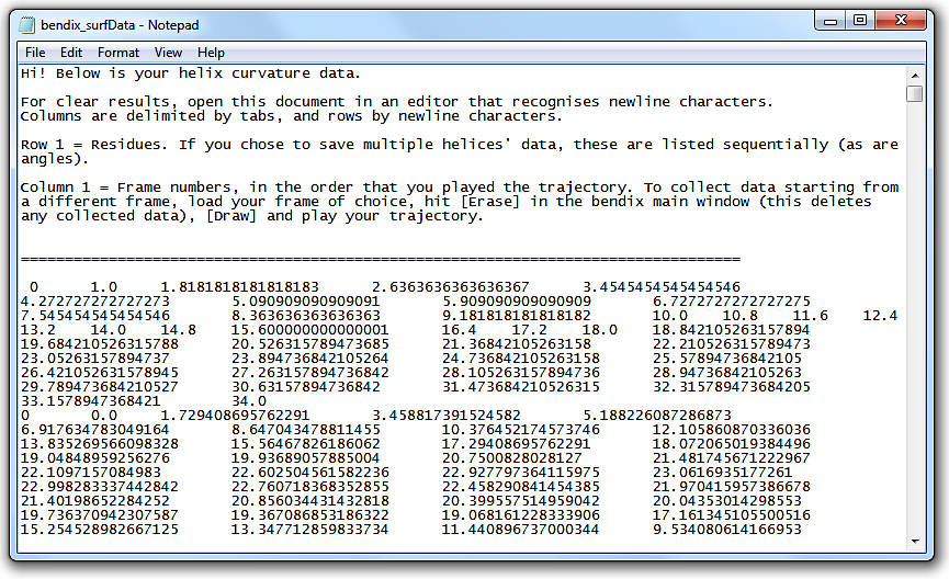
N.B. You do not need to graph data in Angle analysis to export it. Export data from the Bendix main window, under File > Save surf data...
Press Return in the Angle Analysis window to erase your graph and return to your previous protein view.
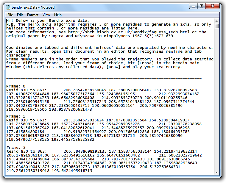
9. Retrieve the helix axis coordinates
You can access the computed axis coordinates for your helix (or helices) of interest.
Axis coordinate data, like helix angle data, is not stored by default, so to switch it on, select
Analysis > Store helix axes.
Redraw your protein and/or replay your trajectory to generate static or dynamic axis coordinate data.
Note that
use every [N] residues determines how many axis points are saved along a helix. Axis points at the end of helices are always stored
(for more information on Bendix' axis generating algorithm, refer to the
Technical details under the faq section).
Write coordinate data to file under
File > Save axes data. Ensure that you use a file extension that you can read.
For a tutorial on VMD, see this website.